Quant Methods · intermediate · 7 min

Confidence Intervals on a Backtest

A backtest hands you a single, confident-looking number for each statistic: Sharpe 0.8, win rate 60%, total return +45%. Each of those is computed from the one sequence of trades that happened to occur. Run the same idea over a slightly different slice of history — or the same history with luck falling differently — and every one of those numbers would move. The single figure hides how much it would move. A confidence interval is the honest version: not "Sharpe 0.8" but "Sharpe 0.8, and 90% of resampled histories land between 0.3 and 1.4."

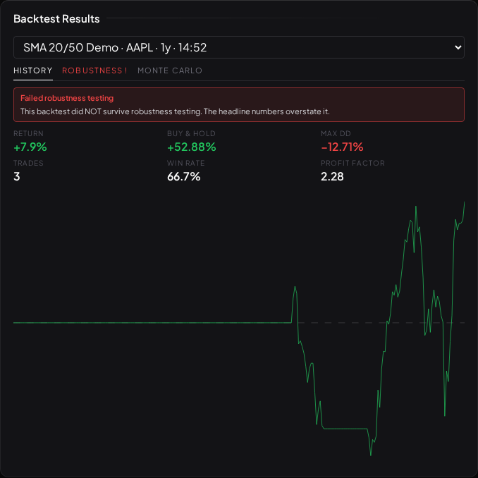
A Backtest Results panel — the point statistics each carry a bootstrapped 90% interval beneath them

The one sample problem

Every statistic on a backtest is an estimate, made from a sample of trades. The sample you got is not the only sample the strategy could have produced; it is one draw from all the ways those trades could have shaken out. The point estimate answers "what happened?" The question that actually matters for trading the strategy forward is "how much does what happened tell me about the strategy?" — and a single number cannot answer that. Two strategies can both post a Sharpe of 0.8: one over 300 trades, one over 8. They are not remotely equally believable, yet the headline number is identical. The missing information is the error around the estimate, and that is exactly what a confidence interval restores.

The bootstrap

You do not need a second history to see how much a number would move — you can manufacture plausible alternative histories from the trades you already have. The technique is the bootstrap:

Take the list of per-trade returns the backtest produced.
Draw a new list of the same length at random, with replacement — some trades appear twice, some not at all. That is one resampled history.
Recompute the statistic (Sharpe, win rate, whatever) on that resampled history.
Repeat a couple of thousand times.

You now have a couple of thousand values of the statistic instead of one — a whole distribution. Sort them and read off the 5th and 95th percentiles, and you have a 90% confidence interval: the middle 90% of the resampled values. Visor does exactly this, with a fixed random seed so the interval is reproducible — the same trades always give the same band.

The width is the point

The single most useful thing about the interval is not where it sits but how wide it is. A narrow band means the statistic is well pinned down: the trades agree with each other, and resampling them barely moves the number. A wide band means the opposite — the sample is small or the trades disagree wildly, and the "estimate" is barely an estimate at all.

This is why a handful of trades should make you nervous, and the interval makes that nervousness visible. Eight trades produce a band so wide it is almost useless — and that width is the honest answer, not a defect to be hidden. A wide confidence interval on a great-looking Sharpe is the chart-level version of the sample-size rule this whole track keeps returning to: a number you cannot repeat is not yet a result. Visor does not dress that up. Below a handful of trades it declines to draw the band at all, for the same reason it declines to render a robustness verdict — there is nothing there to measure yet.

Does the interval clear zero?

For the Sharpe ratio there is one extra reading worth calling out: does the interval include zero? If the 90% band runs from 0.3 to 1.4, it sits entirely above zero — the sample establishes, at that confidence, that the risk-adjusted edge is at least positive. If instead it runs from −0.6 to 1.4, it straddles zero, and the sample has not even settled the sign of the edge, let alone its size. Visor shows this as a plain "Sharpe CI excludes zero: yes/no" line. It is deliberately kept as extra context beside the four robustness gates, not folded into the verdict — a wide band that crosses zero is a caution, not a separate pass-or-fail test.

What the bootstrap assumes — and where it stops

The resampling above draws trades independently of each other. That quietly assumes the order of trades carries no information — that shuffling them changes nothing. For statistics that are just a summary of the whole set of returns — total return, win rate, expectancy, Sharpe — that is fair: reorder the trades and the average, the win count, and the compounded product are all unchanged. Trade returns are also close enough to independent in practice for this to be a defensible null.

It is not fair for everything, and Visor draws the line honestly. Maximum drawdown depends on the order trades arrive in, not just the set of them — a losing streak bunched together digs a far deeper hole than the same losses scattered apart. An independent resample destroys exactly the ordering that drawdown is made of, so a drawdown interval built that way would answer a question it had already thrown away the information for. So the four rows above — total return, win rate, expectancy, Sharpe — get the independent bootstrap, and drawdown does not.

A band for drawdown: the block bootstrap

Refusing the independent resample for drawdown does not mean refusing a band altogether — it means using a resample that keeps the ordering intact. That tool is the block bootstrap. Instead of drawing one trade at a time, it draws short contiguous runs of trades — blocks — and stitches them together into a fresh full-length history:

Pick a block length (Visor uses about √n trades — long enough to hold a real streak, short enough to leave many distinct blocks to draw from).
Draw blocks at random and lay them end to end until you have a full-length history. Because each block is a run of adjacent trades, a cluster of consecutive losers can reappear intact — the streak structure survives.
Compound that history into an equity curve and read off its max drawdown.
Repeat a couple of thousand times, and take the 5th–95th percentiles as before.

The result is an honest 90% band for max drawdown, shown on the backtest panel beneath the four independent-resample rows and labelled with the block length so the assumption is visible. Read it the same way as the others — the width is the point — but with one caveat stated plainly on the panel: it assumes streak structure matters, not the exact order. Reshuffling still happens at the block boundaries, so the block bootstrap answers "how bad could the drawdown be if the streaks fell differently?" rather than pretending the precise sequence is sacred. The path-aware tail-risk view on the Monte Carlo tab remains the companion read: it simulates full ordered equity paths and reports the 95th-percentile drawdown.